Statistics Foundations
This notebook covers the core ideas of applied statistics that we will rely on throughout the course. It is meant for students who have written a little Python but have not seen most of these statistical ideas before.
The aim is to give you a working understanding of:
- The two main branches of statistics: descriptive and inferential.
- Probability, in just enough depth to be useful.
- Random variables, both discrete and continuous.
- Three common probability distributions: Normal, Binomial, and Poisson.
- The Central Limit Theorem.
- Hypothesis testing, p-values, and statistical significance.
Each section is built around a small example with code, a picture, and a short discussion. There are a few short exercises along the way.
Setup
We will use a few standard Python libraries. Install with pip install numpy pandas matplotlib scipy seaborn if needed.
import numpy as np
import pandas as pd
import matplotlib.pyplot as plt
import seaborn as sns
from scipy import stats

sns.set_theme(style="whitegrid")
plt.rcParams["figure.figsize"] = (8, 4)

# A reproducible random number generator.
rng = np.random.default_rng(42)

print("Libraries loaded.")
Libraries loaded.
1. Types of Statistics
Statistics is usually divided into two parts:
| Type | What it does | Example |
|---|---|---|
| Descriptive | Summarises data we already have | "The average exam score in our class was 72." |
| Inferential | Uses a sample to draw conclusions about a larger population | "Based on a survey of 500 students, we estimate that all college students sleep about 6.4 hours a night." |
A useful analogy: descriptive statistics is reporting exactly what is on the pizza in front of you. Inferential statistics is tasting one slice and trying to describe the rest of the pizza you have not seen.
1.1 Descriptive statistics
Suppose we collected the exam scores of 30 students. We want a quick summary.
# Imaginary exam scores out of 100.
exam_scores = rng.normal(loc=72, scale=12, size=30).round().clip(0, 100)
print("Raw scores:", exam_scores.astype(int))

print("\nCentre of the data")
print(f"  Mean   : {np.mean(exam_scores):.2f}")
print(f"  Median : {np.median(exam_scores):.2f}")
print(f"  Mode   : {stats.mode(exam_scores, keepdims=False).mode}")

print("\nSpread of the data")
print(f"  Min, Max : {exam_scores.min():.0f}, {exam_scores.max():.0f}")
print(f"  Range    : {exam_scores.max() - exam_scores.min():.0f}")
print(f"  Std dev  : {np.std(exam_scores, ddof=1):.2f}")
print(f"  Variance : {np.var(exam_scores, ddof=1):.2f}")
Raw scores: [76 60 81 83 49 56 74 68 72 62 83 81 73 86 78 62 76 60 83 71 70 64 87 70
 67 68 78 76 77 77]

Centre of the data
  Mean   : 72.27
  Median : 73.50
  Mode   : 76.0

Spread of the data
  Min, Max : 49, 87
  Range    : 38
  Std dev  : 9.33
  Variance : 86.96
fig, axes = plt.subplots(1, 2, figsize=(11, 4))

axes[0].hist(exam_scores, bins=10, color="#4C72B0", edgecolor="white")
axes[0].axvline(np.mean(exam_scores), color="red", linestyle="--",
                label=f"Mean = {np.mean(exam_scores):.1f}")
axes[0].axvline(np.median(exam_scores), color="green", linestyle=":",
                label=f"Median = {np.median(exam_scores):.1f}")
axes[0].set_title("Distribution of exam scores")
axes[0].set_xlabel("Score")
axes[0].set_ylabel("Number of students")
axes[0].legend()

axes[1].boxplot(exam_scores, vert=False)
axes[1].set_title("Box plot")
axes[1].set_xlabel("Score")

plt.tight_layout()
plt.show()

How to read the box plot:
- The box covers the middle 50% of the data.
- The line inside the box is the median.
- The whiskers reach the typical minimum and maximum.
- Points beyond the whiskers are outliers.
1.2 Inferential statistics
In real studies we cannot measure everyone in the population. We measure a sample and try to say something useful about the population it came from.
| Term | Meaning |
|---|---|
| Population | The whole group we care about (for example, all BSIT students in Nepal). |
| Sample | A subset of the population that we actually measured. |
| Parameter | A numerical property of the population (μ, σ). Usually unknown. |
| Statistic | A numerical property of the sample (x̄, s). What we actually compute. |
The whole game of inferential statistics is summarised by the question:
Given my sample statistic, what can I reasonably say about the unknown population parameter?
# Pretend the true average daily Instagram time across all students is 95 minutes.
# We do not know this in advance; we have to estimate it.
TRUE_POPULATION_MEAN = 95
TRUE_POPULATION_STD  = 25

# Suppose we can survey only 40 students.
sample = rng.normal(TRUE_POPULATION_MEAN, TRUE_POPULATION_STD, size=40)

x_bar = np.mean(sample)
s     = np.std(sample, ddof=1)

print("Our 40-student sample says:")
print(f"  sample mean (x_bar) = {x_bar:.2f} minutes per day")
print(f"  sample std  (s)     = {s:.2f} minutes per day")
print(f"\nThe true population mean (mu) = {TRUE_POPULATION_MEAN} minutes per day, normally unknown.")
print(f"Our estimate is off by {abs(x_bar - TRUE_POPULATION_MEAN):.2f} minutes.")
Our 40-student sample says:
  sample mean (x_bar) = 97.19 minutes per day
  sample std  (s)     = 19.78 minutes per day

The true population mean (mu) = 95 minutes per day, normally unknown.
Our estimate is off by 2.19 minutes.
Quick check.
- "The median age in our class is 19." Descriptive or inferential?
- "Based on 1,000 voters, candidate A is leading nationally." Descriptive or inferential?
- The number 7.2, computed from your 40-student sleep survey, is a parameter or a statistic?
Answers: 1. Descriptive. 2. Inferential. 3. A statistic, since it came from a sample.
2. Probability
Probability is just a number between 0 and 1 expressing how likely something is.
P(event) = 0means impossible.P(event) = 1means certain.P(event) = 0.5means a 50-50 chance, like a fair coin.
The classical formula is
For example, the probability of rolling an even number on a fair six-sided die is 3/6 = 0.5, since {2, 4, 6} are favourable out of {1, 2, 3, 4, 5, 6} possible.
When the maths gets harder, simulation is a useful sanity check.
# Simulate 100,000 die rolls and count how often we get an even number.
n_rolls = 100_000
rolls = rng.integers(low=1, high=7, size=n_rolls)  # values 1..6 inclusive
prob_even = np.mean(rolls % 2 == 0)

print(f"Theoretical P(even) = 0.5")
print(f"Simulated  P(even) = {prob_even:.4f}  (over {n_rolls:,} rolls)")
Theoretical P(even) = 0.5
Simulated  P(even) = 0.4997  (over 100,000 rolls)
As we run more trials, the observed proportion gets closer to the true probability. This is the law of large numbers.
# Watch the running proportion of heads converge to 0.5.
flips = rng.integers(0, 2, size=2000)  # 0 = tails, 1 = heads
running_average = np.cumsum(flips) / np.arange(1, len(flips) + 1)

plt.plot(running_average, color="#4C72B0", label="Observed proportion of heads")
plt.axhline(0.5, color="red", linestyle="--", label="True probability = 0.5")
plt.xlabel("Number of coin flips")
plt.ylabel("Proportion of heads so far")
plt.title("Law of large numbers")
plt.legend()
plt.show()

Two ideas you will see often:
- Independent events are events whose outcomes do not affect each other (for example, two separate coin flips).
- Conditional probability is the probability of A given that B has already happened, written
P(A | B). For example, the probability that a student passes given they studied for at least five hours.
These two ideas underlie a great deal of machine learning, recommender systems, and Bayesian reasoning. We will return to them later.
3. Random Variables
A random variable is a number whose value comes from some random process. Examples:
X = number of likes your post gets in one hourY = your friend's commute time tomorrowZ = whether your code compiles on the first try(1 = yes, 0 = no)
There are two types:
| Type | Values | Examples |
|---|---|---|
| Discrete | Countable: 0, 1, 2, 3, ... | Number of bugs in a program; number of students absent. |
| Continuous | Any value in a range, including decimals | Time spent studying; height; CPU temperature. |
A useful rule of thumb: if you would naturally report it as "5 things", it is discrete. If you would report it as "5.27 seconds", it is continuous.
# Discrete: number of bugs reported per day in a small app.
bugs_per_day = rng.poisson(lam=3, size=200)

# Continuous: time, in hours, students spent on a coding assignment.
study_hours = rng.normal(loc=4.5, scale=1.2, size=200).clip(0, None)

fig, axes = plt.subplots(1, 2, figsize=(12, 4))

# Discrete data: bar chart of counts.
unique, counts = np.unique(bugs_per_day, return_counts=True)
axes[0].bar(unique, counts, color="#DD8452", edgecolor="white")
axes[0].set_title("Discrete: bugs per day")
axes[0].set_xlabel("Number of bugs")
axes[0].set_ylabel("Days")

# Continuous data: histogram.
axes[1].hist(study_hours, bins=20, color="#55A868", edgecolor="white")
axes[1].set_title("Continuous: hours spent on assignment")
axes[1].set_xlabel("Hours")
axes[1].set_ylabel("Number of students")

plt.tight_layout()
plt.show()

print(f"Average bugs per day  : {bugs_per_day.mean():.2f}")
print(f"Average study hours   : {study_hours.mean():.2f}")

Average bugs per day  : 3.02
Average study hours   : 4.38
4. Common Distributions
A distribution describes how the values of a random variable are spread out. Three are particularly important.
4.1 The Normal distribution
The Normal distribution is the familiar bell curve. It tends to appear when many small random effects add up. Heights, exam scores, measurement errors, and many other quantities are roughly Normal.
A useful rule of thumb (the 68-95-99.7 rule):
- About 68% of values lie within one standard deviation of the mean.
- About 95% lie within two standard deviations.
- About 99.7% lie within three standard deviations.
We write X ~ Normal(mu, sigma), where mu is the mean and sigma is the standard deviation.
# Simulating exam scores with mean 70 and standard deviation 10.
mu, sigma = 70, 10
scores = rng.normal(mu, sigma, size=10_000)

x = np.linspace(30, 110, 200)
pdf = stats.norm.pdf(x, mu, sigma)

plt.hist(scores, bins=40, density=True, color="#4C72B0", alpha=0.6,
         label="Simulated scores")
plt.plot(x, pdf, "r-", lw=2, label=f"Normal(mu={mu}, sigma={sigma})")
plt.fill_between(x, pdf, where=(x >= mu - sigma) & (x <= mu + sigma),
                 alpha=0.3, color="orange", label="Within 1 std dev (~68%)")

plt.title("Normal distribution: exam scores")
plt.xlabel("Score")
plt.ylabel("Density")
plt.legend()
plt.show()

inside = np.mean(np.abs(scores - mu) <= sigma)
print(f"Fraction of simulated scores within 1 std dev (theory ~ 0.68): {inside:.3f}")

Fraction of simulated scores within 1 std dev (theory ~ 0.68): 0.687
4.2 The Binomial distribution
Use the Binomial distribution when you repeat the same experiment n times, each trial has only two outcomes (success or failure), and the trials are independent. Some examples:
- Out of 10 coin flips, how many come up heads?
- Out of 50 app installs, how many users open the app at least once?
- Out of 20 quiz questions, how many do you get right by guessing?
We write X ~ Binomial(n, p), where n is the number of trials and p is the probability of success on each trial. The mean is n * p and the variance is n * p * (1 - p).
# Suppose our app crashes on launch with probability 0.30.
# Out of 20 launches, how many crashes do we expect?
n, p = 20, 0.30

k = np.arange(0, n + 1)
pmf = stats.binom.pmf(k, n, p)

# Simulate 10,000 sets of 20 launches.
sims = rng.binomial(n, p, size=10_000)

fig, axes = plt.subplots(1, 2, figsize=(12, 4))

axes[0].bar(k, pmf, color="#C44E52", edgecolor="white")
axes[0].set_title(f"Theoretical Binomial(n={n}, p={p})")
axes[0].set_xlabel("Number of crashes")
axes[0].set_ylabel("Probability")

axes[1].hist(sims, bins=np.arange(-0.5, n + 1.5), density=True,
             color="#8172B2", edgecolor="white")
axes[1].set_title("10,000 simulated runs")
axes[1].set_xlabel("Number of crashes")

plt.tight_layout()
plt.show()

print(f"Expected number of crashes (n*p): {n * p:.2f}")
print(f"Average from the simulation     : {sims.mean():.2f}")
print(f"P(exactly 6 crashes)            : {stats.binom.pmf(6, n, p):.4f}")
print(f"P(more than 8 crashes)          : {1 - stats.binom.cdf(8, n, p):.4f}")

Expected number of crashes (n*p): 6.00
Average from the simulation     : 6.01
P(exactly 6 crashes)            : 0.1916
P(more than 8 crashes)          : 0.1133
4.3 The Poisson distribution
The Poisson distribution counts how many times something happens in a fixed window, when the events are rare and roughly independent. For example:
- Notifications received per hour.
- Customers entering a shop per minute.
- Bugs reported on a project per day.
We write X ~ Poisson(lambda), where lambda is the average number of events per window. For a Poisson distribution the mean and the variance are both equal to lambda.
# On average, eight social media notifications per hour.
lam = 8
k = np.arange(0, 25)
pmf = stats.poisson.pmf(k, lam)
sims = rng.poisson(lam, size=10_000)

fig, axes = plt.subplots(1, 2, figsize=(12, 4))

axes[0].bar(k, pmf, color="#937860", edgecolor="white")
axes[0].axvline(lam, color="red", linestyle="--", label=f"lambda = {lam}")
axes[0].set_title("Theoretical Poisson(lambda=8)")
axes[0].set_xlabel("Notifications in 1 hour")
axes[0].set_ylabel("Probability")
axes[0].legend()

axes[1].hist(sims, bins=np.arange(-0.5, 25.5), density=True,
             color="#DA8BC3", edgecolor="white")
axes[1].set_title("10,000 simulated hours")
axes[1].set_xlabel("Notifications in 1 hour")

plt.tight_layout()
plt.show()

print(f"P(0 notifications next hour) = {stats.poisson.pmf(0, lam):.4f}")
print(f"P(15 or more notifications)  = {1 - stats.poisson.cdf(14, lam):.4f}")

P(0 notifications next hour) = 0.0003
P(15 or more notifications)  = 0.0173
Try it yourself.
- In the Binomial cell, change
pto0.05and re-run. The shape becomes much more skewed towards zero. - In the Poisson cell, set
lamfirst to2, then to30. Aslambdagrows, the shape starts to look like a bell curve. The next section explains why.
5. The Central Limit Theorem
The Central Limit Theorem (CLT) is one of the most important results in statistics:
If you take many samples from any distribution and look at the distribution of the sample means, those means form a Normal distribution, even if the original data was nothing like a bell curve.
The conditions are mild:
- The samples are independent.
- The sample size is reasonably large. In practice,
n >= 30is usually enough.
Why this matters
Most formulas in inferential statistics, including confidence intervals and hypothesis tests, assume that some quantity is approximately Normal. The CLT is what makes that assumption work in practice. It is the reason the same t-test can be applied to wait times, app session lengths, weights of mangoes, and so on, even though those quantities individually look very different.
# Start with a clearly non-Normal population: an exponential distribution,
# which is heavily skewed to the right.
population = rng.exponential(scale=5.0, size=100_000)

plt.hist(population, bins=60, color="#C44E52", edgecolor="white")
plt.title("Original population (exponential, skewed)")
plt.xlabel("Value")
plt.ylabel("Count")
plt.show()

print(f"Population mean: {population.mean():.2f}")
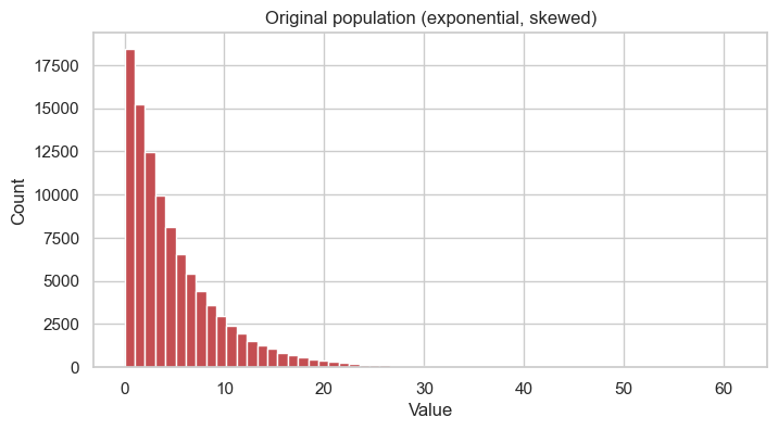
Population mean: 4.99
# Take many random samples, compute their means, and plot the distribution
# of those sample means for different sample sizes.

def plot_clt(sample_size, n_samples=2000, ax=None):
    means = [rng.choice(population, size=sample_size, replace=False).mean()
             for _ in range(n_samples)]
    ax.hist(means, bins=40, color="#4C72B0", edgecolor="white", density=True)
    ax.set_title(f"Sample means (n={sample_size})")
    ax.set_xlabel("Sample mean")
    ax.axvline(np.mean(means), color="red", linestyle="--",
               label=f"average = {np.mean(means):.2f}")
    ax.legend()

fig, axes = plt.subplots(1, 4, figsize=(16, 4))
for ax, n in zip(axes, [2, 5, 30, 100]):
    plot_clt(n, ax=ax)

plt.suptitle("Central Limit Theorem: as n grows, sample means become Normal", y=1.02)
plt.tight_layout()
plt.show()

Three things to notice:
- The original data was strongly skewed, but the distribution of sample means quickly takes on a bell shape.
- As the sample size
ngrows, the bell becomes narrower; that is, the sample mean becomes a more reliable estimate of the population mean. - The centre of the distribution of sample means lines up with the true population mean.
This is the reason that statements like "average users spend 27 minutes a day, plus or minus about 2 minutes" are trustworthy, even when individual users vary widely.
6. Hypothesis Testing, p-values, and Significance
Hypothesis testing is the formal way of asking the following question:
Is what I am seeing in the data a real effect, or could it be explained by random chance?
The five-step recipe
- State two competing claims:
- H₀ (null hypothesis): the boring, default explanation, for example "no change".
- H₁ (alternative hypothesis): the interesting claim, for example "things are different".
- Pick a significance level α, commonly 0.05. This is the risk of a false alarm we are willing to accept.
- Collect data and compute a test statistic.
- Compute the p-value: assuming H₀ is true, the probability of observing data at least as extreme as what we got.
- Decide:
- If p < α, reject H₀. The result is statistically significant.
- Otherwise, do not reject H₀. There is not enough evidence to overturn the default.
A familiar analogy from programming
- H₀: the new code is no faster than the old code.
- H₁: the new code is faster.
- p-value: assuming the two versions are really the same speed, how often would we see a speed-up at least as large as the one we measured?
If that probability is very small, the speed-up is unlikely to be a coincidence.
A worked example
Suppose the typical time to solve a debugging exercise is 20 minutes. We let 25 students drink a cup of coffee and then time them on the same exercise. Their average time turns out to be 18.4 minutes.
Is the coffee really helping, or could 18.4 minutes have arisen by chance?
- H₀: mu = 20 (coffee makes no difference).
- H₁: mu < 20 (coffee makes students faster). This is a one-sided test.
- α = 0.05.
# Generate the timing data for the coffee group.
coffee_times = rng.normal(loc=18.4, scale=4.0, size=25)
print("Coffee group times (minutes):")
print(np.round(coffee_times, 1))

claimed_mean = 20  # the no-effect baseline (H0)

# scipy gives us the two-sided result; we adjust for a one-sided test.
t_stat, p_two_sided = stats.ttest_1samp(coffee_times, popmean=claimed_mean)
p_one_sided = p_two_sided / 2 if t_stat < 0 else 1 - p_two_sided / 2

print(f"\nSample mean        : {coffee_times.mean():.2f} minutes")
print(f"Sample std         : {coffee_times.std(ddof=1):.2f}")
print(f"t-statistic        : {t_stat:.3f}")
print(f"p-value (one-sided): {p_one_sided:.4f}")

alpha = 0.05
if p_one_sided < alpha:
    print(f"\np = {p_one_sided:.4f} < alpha = {alpha}")
    print("We reject H0. There is evidence that coffee speeds up debugging.")
else:
    print(f"\np = {p_one_sided:.4f} >= alpha = {alpha}")
    print("We do not reject H0. The apparent speed-up could be random noise.")
Coffee group times (minutes):
[20.3 27.3 19.7 18.2 19.9 18.  21.8 21.2 23.  22.3 15.8 21.  21.6 13.8
 21.8 15.  18.1 19.8 19.2 15.6 23.  14.6 16.8 19.5 22.5]

Sample mean        : 19.58 minutes
Sample std         : 3.18
t-statistic        : -0.656
p-value (one-sided): 0.2590

p = 0.2590 >= alpha = 0.05
We do not reject H0. The apparent speed-up could be random noise.
# Where does our t-statistic fall in the t-distribution?
x = np.linspace(-4, 4, 400)
y = stats.t.pdf(x, df=24)
critical = stats.t.ppf(0.05, df=24)  # left-tail critical value at alpha = 0.05

plt.plot(x, y, "b-", label="t-distribution (df=24)")
plt.fill_between(x, y, where=x <= critical, color="red", alpha=0.3,
                 label="Rejection region (alpha=0.05)")
plt.axvline(t_stat, color="black", linestyle="--",
            label=f"Our t = {t_stat:.2f}")
plt.title("Does our t-statistic fall in the rejection region?")
plt.xlabel("t value")
plt.ylabel("Density")
plt.legend()
plt.show()

What a p-value really means
A p-value is the probability of seeing data at least as extreme as what we observed, assuming the null hypothesis is true.
It is not:
- The probability that H₀ is true.
- The probability that we are wrong.
- A measure of how important the effect is. With enough data, even a tiny effect can produce a small p-value.
Two kinds of mistakes
| Reality \ Decision | Reject H₀ | Do not reject H₀ |
|---|---|---|
| H₀ is true | Type I error (false alarm) | Correct |
| H₀ is false | Correct | Type II error (missed effect) |
The significance level α controls the rate of Type I errors. Choosing α = 0.05 means we are willing to accept a 5% chance of crying wolf.
Quick check.
- You run an A/B test on a new sign-up button. The p-value is 0.03 and α is 0.05. What do you do?
- Someone says, "p = 0.20 means there is an 80% chance the new feature works." Is this correct?
- You repeat your experiment 100 times where there is no real effect. With α = 0.05, roughly how many times will you get a "significant" result purely by chance?
Answers: 1. Reject H₀ and adopt the new button. 2. No: a p-value is never the probability that a hypothesis is true. 3. About five.
7. Exercises
These are short exercises to practice the ideas above. Each one has a small starter cell with the structure already laid out.
Exercise 1 - Phone screen time
Generate 60 imaginary "minutes of phone screen time per day" values from a Normal distribution with mean 200 and standard deviation 45. Compute the mean, median, and standard deviation of your sample, and plot a histogram.
Exercise 2 - Quiz guessing
A multiple-choice quiz has 15 questions, each with 4 options. If you guess every answer at random, what is the probability of getting at least 8 correct? Use the Binomial distribution.
Exercise 3 - The CLT for dice rolls
Roll a fair six-sided die. Take samples of size 50. Compute the mean of each sample. Repeat this 1,000 times and plot the distribution of those means. Notice that they are roughly Normal, even though a single die roll is not.
Exercise 4 - A hypothesis test
You suspect that students at your college sleep less than the national average of 7 hours. You survey 30 students and find a sample mean of 6.4 hours with a standard deviation of 1.1. Run a one-sided t-test. Is the difference statistically significant at α = 0.05?
# Exercise 1: phone screen time
# screen_time = rng.normal(loc=..., scale=..., size=...)
# print("Mean   :", ...)
# print("Median :", ...)
# print("Std    :", ...)
# plt.hist(...); plt.show()
# Exercise 2: quiz guessing
# n, p = 15, 1/4
# prob_at_least_8 = 1 - stats.binom.cdf(..., n, p)
# print(prob_at_least_8)
# Exercise 3: CLT for dice
# means = []
# for _ in range(1000):
#     sample = rng.integers(1, 7, size=50)
#     means.append(sample.mean())
# plt.hist(means, bins=30); plt.show()
# Exercise 4: sleep hypothesis test
# sleep = rng.normal(6.4, 1.1, 30)
# t_stat, p_two = stats.ttest_1samp(sleep, popmean=7)
# p_one = p_two / 2 if t_stat < 0 else 1 - p_two / 2
# print("t =", t_stat, "  p (one-sided) =", p_one)
8. Summary and what comes next
In this notebook we covered:
- Descriptive vs inferential statistics: summarising what we have, and inferring what we do not.
- Probability: the basic language of uncertainty.
- Random variables: discrete (countable) and continuous (measurable).
- Distributions: Normal, Binomial, and Poisson.
- The Central Limit Theorem: why averages tend to be Normal.
- Hypothesis testing and p-values: a structured way to separate signal from noise.
These ideas show up everywhere in computing:
| Concept | Where it appears |
|---|---|
| Descriptive statistics | Dashboards, reporting, analytics |
| Probability | Machine learning, recommender systems, spam filters |
| Distributions | Performance benchmarking, simulations, risk analysis |
| Central Limit Theorem | Confidence intervals around metrics |
| Hypothesis testing | A/B testing, quality control, research studies |
In the rest of the course we will build on these foundations:
- Parameter estimation: how models actually learn their parameters from data.
- Linear regression: predicting numbers.
- Regularisation and model metrics: building models that generalise to new data.
The single best way to make these ideas stick is to run the cells, change the numbers, and see what happens. Statistics becomes much easier to understand once you have simulated it a few times.